AWS Redshift Optimization – A Case Study

AWS Redshift – An Overview

Amazon Redshift is a fast, fully managed, petabyte-scaled data warehouse solution that uses columnar storage to minimize Input/Output (I/O), provide high data compression rates, and offer fast performance. As a typical Data Warehouse, it is primarily designed for Online Analytic Processing (OLAP) and Business Intelligence (BI) and not designed to be used as an Online Transaction Processing (OLTP) tool. It supports ANSI-SQL and is a massively parallel processing database.

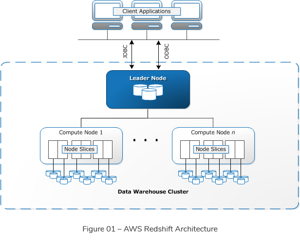
Redshift architecture (See Figure 01) consists of a tightly coupled EC2 Compute nodes cluster. The Redshift cluster is built on a single availability zone in order to negate any network latency issue between availability zones. Having all nodes in close proximity will reduce network latency and will improve performance.

Users can create one or more clusters with each cluster having multiple databases. Most of the time there is one Redshift cluster and additional clusters can be added for resilience purposes. Any cluster can have two types of nodes, namely a leader node and compute nodes.

The leader node facilitates the communication between the BI client and the compute nodes. Each leader node has a SQL end point. It coordinates the parallel query execution. When a request comes to the leader node, it parses the query and generates an execution plan and a compiled code to be executed in the compute nodes.

The compute nodes process the incoming requests in parallel. Each compute node has a dedicated CPU, memory and a storage. Each compute node can scale out/in and scale up/down (resizing the Redshift cluster). Each compute node consists of slices. The slices are portions of memory and disk. The data is loaded to the slices in parallel. It has a “shared nothing” architecture. All compute nodes are independent of each other and there is no contention between nodes.

Redshift can decide automatically how the data distributes between slices. Also a user can specify one column as the distribution key. When a query is executed, the query optimizer on the leader node redistributes the data on the compute nodes as needed in order to perform any joins and aggregations.

The Challenge

With time, as you load more and more data and apply DML commands, the performance can deteriorate. A US client from the healthcare sector wanted to apply best practices on to their Redshift cluster in order to speed up and improve its performance.

How Auxenta Helped

Leveraging Auxenta’s Redshift expertise, the team proposed a set of best practices and optimization strategies for the client’s Redshift cluster installation.

The Solution

The given Redshift cluster was analyzed based on the following key indicators.

Table Design
Sort keys
Compression
Analyze
Vacuum
Primary and foreign keys

Query Design
Queries with alerts
Queries affected by work load management (WLM) configurations
Tables being used in queries with maximum impact on query performance
Percentage of queries being affected by tables
Tables scanned in select join queries
Select queries in peak CPU usage
Tables using peak CPU usage

WLM Management
Queue resources hourly
Queue resources hourly with CPU usage
Query patterns per user/group
WLM configurations for Redshift

Benefits to the client

Identify the causes and performance drawbacks in the Redshift cluster
Guidelines for improvement
Gaining a good knowledge about Redshift optimization knowledge

References

Ishara Nuwan Karunathilake

Senior Tech Lead